This article is part of a series on Math for Machine Learning, follow along to learn more about some of the math involved with ML
This is a concept that you study once, and expect to remember it for life. But fate has it, you really cannot. I’ve been out in this cycle for over 2 years.
So, now finally I’m nailing this concept down in my blog.
What is a random variable ?
First of all, nothing about a random variable is random :)
It’s essentially a variable used to represent an outcome of an random experiment (e.g. Get a 1 after rolling a die, here 1 is a random variable).
A random variable is not random, but an experiment is.
Types of random variables
- Discrete random variable - Outcome of event is finite (e.g. Getting one of the faces of the die)
- Continuous random variable - Outcome of event is infinite (e.g. Choosing a real number between 0 and 1)
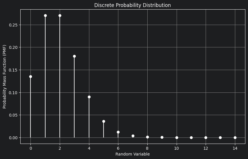
Discrete random variable
- Probability mass function (PMF)
$$
P_X(x) = P(X = x) = p(x)
$$
- It’s just probabilities assigned to random variables
- Some properties: $$ P_X(x) \geq 0 $$ $$ \sum_xP_X(x) = 1 $$
- Cumulative mass function (CMF)
$$
F_X(x) = P(X \leq x) = \sum_{i=-\infty}^xp(x)
$$
- It kinda helps to find probabilites between ranges easily, which would be rather difficult with just PMF $$ P(a\leq X \leq b) = F_X(b) - F_X(a) $$
- Expectation
$$
E[X] = \sum_x xP_X(x)
$$
- It gives you the mean outcome of a random experiment
- Properties: $$ E[aX + b] = aE[X] + b $$
- Variance
$$
Var[X] = E[(X - E[X])^2] = E[X^2] - (E[X])^2
$$
- This measures the spread of the data about the mean
- Properties $$ Var[aX + b] = a^2Var[x] + 0 $$
Continuous random variable
Having understood the discrete random variable, understanding the continuous random variable is pretty easy.
Statisticians are going to hate me for saying this but,
Just replace all summations in the discrete case with integration and you’re good to go
- Probability density function (PDF)
- A continuous random variable is characterized by a probability density function $f_X(x)$
- The probability in a PDF can be defined for only a range, and not for a single random variable $$ P(a \leq X \leq b) = \int_a^bf_X(x) dx $$
- For continuous random variable, $$ P(X = x) = 0 $$
- To conclude, in PDF probability assigned to intervals not points
- Cumulative density function
- A cumulative density function is similar to CMF $$ F_X(x) = P(X \leq x) = \int_{-\infty}^xf_X(x) $$
- PDF and CDF are actually related $$ f_X(x) = \frac{d}{dx}F_X(x) $$
- Expectation $$ E[X] = \int_{-\infty}^{\infty} xP_X(x) $$
- Variance $$ Var[X] = E[(X - E[X])^2] = E[X^2] - (E[X])^2 $$
Discrete Probability Distributions
The probability distributions that follow the discrete random variables are called discrete probability distributions.
- Bernoulli Distribution
- It’s a simple success or failure experiment
- PMF $$ P_X(1) = p $$ $$ P_X(0) = 1-p $$
- Here, 1 means success, 0 means failure, and p is the success probability
- $E[X] = p$
- $Var[X] = p(1-p)$
- Binomial Distribution
- You perform bernoulli trial n times, so you have k successes and n-k failures
- PMF $$ P_X(k) = \binom{n}{k}p^k(1-p)^{n-k} $$
- $E[X] = np$
- $Var[X] = np(1-p)$
A bag contains 5 white balls and 10 black balls. In a random experiment, n balls are drawn from the bag one at a time with replacement. Let Sn denote the total number of black balls drawn in the experiment. The expectation of $S_{100}$ denoted by E[$S_{100}$] = ___
Solution
The above problem follows the binomial distribution.
The number of trials $n = 100$
Success probability $p = \frac{10}{15} = \frac{2}{3}$
So, now we know from the above formulas that $E[S_{100}] = np = 100 \times \frac{2}{3} = 66.67$ - Poisson Distribution
- It’s essentially binomial with infinite number of trials $(n\rightarrow\infty)$ and with the success probability $p$ close to zero
- Let’s understand with an example, let’s say you are a call operator and you get 2 calls per minute on an average.
- Now, here we know something expected number of calls in a minute is 2 and let’s denote it by $\lambda$
- $E[X] = \lambda$, where $X$ denotes number of calls in minute
- Now, I ask the rare case: “What’s the probability that you get 5 calls in a minute ?”
- This qn is rare because on an average we only get 2 calls per minute, so getting 5 is rare. This is the kind of qn Poisson answers
- Poisson’s distribution models extremely rare ($p$ close to 0), it does this by resolving the minutes to seconds, microseconds, nanoseconds…till infinity ($n\rightarrow\infty$)
- PMF $$ P_X(k) = \frac{e^{-\lambda}\lambda^k}{k!} $$
- For our above example, the above equation gives us the probability that k calls happen per minute given that we get only $\lambda$ calls per minute
- For Poisson,
$$
E[X] = Var[X] = \lambda
$$
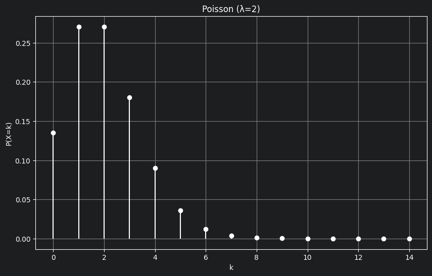
- In the above graph, you can clearly see the probability of the average phone calls being made is maximum, as we move away from the average, our probability closely moves towards zero.
- Discrete Uniform Distribution
- All outcomes are equally likely, like getting a face on rolling a die
- Each face has probability $\frac{1}{6}$
- Expectation $$ E[X] = \frac{a + b}{2} $$
Continuous Distributions
The probability distributions that follow the continuous random variable are called continuous probability distributions.
- Continuous Uniform Distribution (a, b)
- All outcomes with in an interval $[a, b]$ are equally likely
- $X$ can be any real number within this interval $[a, b]$
- PDF $$ f_X(x) = \frac{1}{b-a}, \ a \leq x \leq b $$
- Expectation $$ E[X] = \frac{a + b}{2} $$
- Variance $$ Var[X] = \frac{(b-a)^2}{12} $$
- Exponential Distribution ($\lambda$)
- Used for waiting times
- PDF $$ f_X(x) = \lambda e^{-\lambda x} $$
- CDF $$ F_X(x) = 1 - e^{-\lambda x} $$
- Mean $$ E[X] = \frac{1}{\lambda} $$
- Variance $$ Var[X] = \frac{1}{\lambda^2} $$
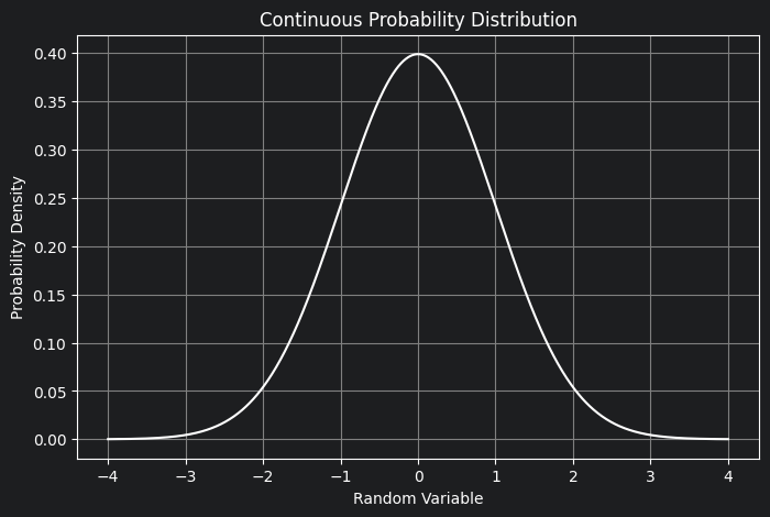
- Normal Distribution ($\mu, \ \sigma^2$)
- Symmetric bell curve
- PDF $$ f_X(x) = \frac{1}{\sqrt{2\pi\sigma^2}}e^{-\frac{(x-\mu)^2}{2\sigma^2}} $$
- Expectation $$ E[X] = \mu $$
- Variance $$ Var[X] = \sigma^2 $$
- Standard Normal
- A popular standardization technique in machine learning $$ Z = \frac{X - \mu}{\sigma} $$
- Mean = 0
- Variance = 1
In the works, but will be completed soon :) HAPPY LEARNING !